

Forewords
This is the first in a data science blog series that I’m writing. My goal for this series is not only sharing, tutorializing, but also, making personal notes while learning and working as a Data Scientist. If you are reading this blog, please feel free to give me any feedback or question you might have.
Note: The source codes as well as original datasets for this series will also be updated at this Github repository of mine.
Preparation
For the purpose of this project, I’m going to use this SkillCraft data set. (You can also download as well as have a quick look of it from this ShareCSV url - Many thanks to Ken Tran and Huy Nguyen for such a neat tool!)
-
Input: StarCraft 2 dataset (CSV) with 20 different attributes.
-
Output: A classification / prediction model to determine League Index (more information and context can be found here
-
Prerequisites: Python (with Pandas and Scikit-learn), iPython Notebook (as an awesome IDE), Unix Shell Script.
In Action
Step 1: Clean the data. I’m going to use a simple Bash script for this.
- As you can see: there is some “missing-value” entries - denoted as “?”:
$ cat SkillCraft1_Dataset.csv | grep "?" | head -2
1064,5,17,20,"?",94.4724,0.0038460052,0.0007827297,3,"9.66332959684589e-06",0.0001352866,0.0044741216,50.5455,54.9287,3.0972,31,0.0007634,7,0.0001062966,0.00011596
5255,5,18,"?","?",122.247,0.0063568492,0.0004328068,3,"1.35252109932915e-05",0.000256979,0.0030431725,30.8929,62.2933,5.3822,23,0.001055,5,0,0.00033813- A 1-liner bash script to clean them up:
$ sed '/?/d' SkillCraft1_Dataset.csv > SkillCraft1_Dataset_clean.csvStep 2: Load and prepare the dataset. We will use iPython Notebook from now.
- Load:
import pandas as pd
df = pd.read_csv('./Dataset/Starcraft/SkillCraft1_Dataset_clean.csv')- Divide the given data set into Train (75%) and Test (25%) sets:
df['is_train'] = np.random.uniform(0, 1, len(df)) <= .75
train_df, test_df = df[df['is_train']==True], df[df['is_train']==False]
Step 3: Apply Machine Learning algorithm.
- We will use Random Forest classification for this example:
from sklearn.ensemble import RandomForestClassifier- Chose the features set:
features = ["APM","Age","TotalHours","UniqueHotkeys", "SelectByHotkeys", "AssignToHotkeys", "WorkersMade","ComplexAbilitiesUsed","MinimapAttacks","MinimapRightClicks"]- Define your classifier and train it: (n_estimators is the number of trees in your forest, in this case I would just use 10.)
rfc = RandomForestClassifier(n_estimators=10)
rfc.fit(train_df[list(features)], train_df.LeagueIndex)
Step 4: Evaluations:
pd.crosstab(test_df.LeagueIndex, rfc.predict(test_df[features]), rownames=["Pred"], colnames=["Actual"])RandomForestClassifier
Actual 1 2 3 4 5 6 7
Pred
1 17 18 7 4 0 0 0
2 14 22 20 19 7 1 0
3 8 28 33 64 18 4 0
4 9 14 41 86 61 17 0
5 0 6 16 58 66 45 0
6 0 0 3 25 47 73 0
7 0 0 0 0 3 5 1We can see that the correctness reduce greatly at League #1 and #7. It’s simply because they are the 2 classes with lowest number of members. With a little over 3000 entries in our given dataset, we simply don’t have enough data to “learn”.
- Plot it!
pd.crosstab(test_df.LeagueIndex, rfc.predict(test_df[features]), rownames=["Pred"], colnames=["Actual"]).plot()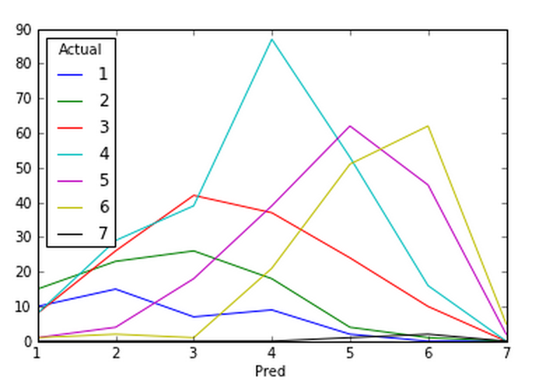
- RMSD:
np.sqrt(sum(pow(test_df.LeagueIndex - classifier.predict(test_df[features]),2)) / float(len(test_df)))>1.23877447987##Conclusions##
- With the above (relatively confident) result, we can already see the benefit of using data science in a simple classification problem.
- There are, of course, a few ways to improve our result: Larger dataset. 3000 entries is simply not enough for this model. Better dataset. We would love to get a dataset with an even distribution of League members. For Random Forest, simply improving our features set in quality and quantity, or increasing the number of trees would give us a better result at a certain performance cost. Consider different classifiers (described below).
##Take it to another level## Now that we’ve used a proper classification technique (Random Forest), but that’s not everything about data science. Choosing the right technique for the right task is not only an interesting problem, but also mandatory. In this part, we are going to compare between various classifiers and pick the best one for the task:
- Mass-define classifiers:
from sklearn.ensemble import ExtraTreesClassifier, RandomForestClassifier
from sklearn.neighbors import KNeighborsClassifier
from sklearn.lda import LDA
from sklearn.qda import QDA
from sklearn.naive_bayes import GaussianNB
from sklearn.tree import DecisionTreeClassifier

classifiers = [
    ExtraTreesClassifier(n_estimators=10),
    RandomForestClassifier(n_estimators=10),
    KNeighborsClassifier(100),
    LDA(),
    QDA(),
    GaussianNB(),
    DecisionTreeClassifier()
]- Train them:
import time
features = ["APM","Age","TotalHours","UniqueHotkeys", "SelectByHotkeys", "AssignToHotkeys",
            "WorkersMade","ComplexAbilitiesUsed","MinimapAttacks","MinimapRightClicks" ]

for classifier in classifiers:
    print classifier.class.name
    start = time.time()
    classifier.fit(train_df[list(features)], train_df.LeagueIndex)
    print "  -> Training time:", time.time() - start
ExtraTreesClassifier
-> Training time: 0.0490028858185
RandomForestClassifier
-> Training time: 0.0870010852814
KNeighborsClassifier
-> Training time: 0.00781583786011
LDA
-> Training time: 0.0202190876007
QDA
-> Training time: 0.00545406341553
GaussianNB
-> Training time: 0.00332403182983
DecisionTreeClassifier
-> Training time: 0.0392520427704- Evaluation:
for classifier in classifiers:
    print classifier.__class__.__name__
    print np.sqrt(sum(pow(test_df.LeagueIndex - classifier.predict(test_df[features]),2)) / float(len(test_df)))
ExtraTreesClassifier
1.2280633269
RandomForestClassifier
1.19202778179
KNeighborsClassifier
1.23231678199
LDA
1.1164728514
QDA
1.55181813847
GaussianNB
1.49456379263
DecisionTreeClassifier
1.38093328738As we can see, Linear Discriminant Analysis (LDA) clearly won with a relatively low training time and best RMSD!