Minimal Data Science #2: Avazu CTR Prediction with Scikit-learn and Amazon Machine Learning

TL;DR: Results, Pros and Cons

Introduction

This is the second post of my Minimal Data Science blog series, the first post can be located at lenguyenthedat.github.io/minimal-data-science-1-starcraft. My goal for this series still, is not only sharing, tutorializing, but also, making personal notes while learning and working as a Data Scientist. If you are reading this blog, please feel free to give me any feedback or question you might have.

In this post, we will be looking into one of those classic Kaggle challenges - the Avazu CTR Prediction challenge, describing how I have built a working solution for it - with acceptable result. I will also try to solve it with Amazon’s new Machine Learning service.

Note: The source codes as well as original datasets for this series will also be updated at this Github repository of mine.

The Challenge

As described in Avazu CTR Prediction challenge.

The problem can be summarized as:

• We are given data set consists of huge number of user sessions which, was described by a number of variables:
  • Identified variables (ids,timestamp,site metadata, application metadata, devices)
  • Anonymized variables (C1, C14-C21)
  • A single target (binary) variable (click), that was available in the training data set, and hidden from the test data set.
• The goal is to predict the probability of user clicking for given sessions.
• Submission should include all session IDs and their click chance.
• Evaluation method: Logarithmic Loss (Logarithmic Loss can also be calculated from the following built-in function in Scikit-Learn)

Preparation

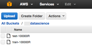
For simplicity, I’ve pre-processed a smaller version (1M randomed entries) of training and test data set at this chapter’s Github repo. The 2 files were also uploaded into a separated S3 bucket for Amazon Machine Learning (AML) service to use.

Scikit Learn

I won’t be going into too much detail about my implementation this time, it should be quite similar to what we have gone through in this series’ first post. Below, however, are a few pre-process steps that I’ve done in order to achieve better model:

Normalizing values with StandardScaler and LabelEncoder:

from sklearn.preprocessing import StandardScaler, LabelEncoder

le = LabelEncoder()
for col in ['site_id','site_domain','site_category','app_id','app_domain',
            'app_category','device_model','device_id','device_ip']:
    le.fit(list(train[col])+list(test[col]))
    train[col] = le.transform(train[col])
    test[col] = le.transform(test[col])

scaler = StandardScaler()
for col in ['C1','banner_pos','device_type','device_conn_type',
            'C14','C15','C16','C17','C18','C19','C20','C21']:
    scaler.fit(list(train[col])+list(test[col]))
    train[col] = scaler.transform(train[col])
    test[col] = scaler.transform(test[col])

Feature engineering:

train['day'] = train['hour'].apply(lambda x: (x - x%10000)/1000000) # day
train['dow'] = train['hour'].apply(lambda x: ((x - x%10000)/1000000)%7) # day of week
train['hour'] = train['hour'].apply(lambda x: x%10000/100) # hour
test['day'] = test['hour'].apply(lambda x: (x - x%10000)/1000000) # day
test['dow'] = test['hour'].apply(lambda x: ((x - x%10000)/1000000)%7) # day of week
test['hour'] = test['hour'].apply(lambda x: x%10000/100) # hour

Removing outliners:

for col in ['C18','C20','C21']:
    # keep only the ones that are within +3 to -3 standard deviations in the column col,
    train = train[np.abs(train[col]-train[col].mean())<=(3*train[col].std())]
    # or if you prefer the other way around
    train = train[~(np.abs(train[col]-train[col].mean())>(3*train[col].std()))]

Output:

ExtraTreesClassifier
  -> Training time: 25.1661880016
RandomForestClassifier
  -> Training time: 56.4664750099
KNeighborsClassifier
  -> Training time: 2.17064404488
LDA
  -> Training time: 0.327888965607
GaussianNB
  -> Training time: 0.166214227676
DecisionTreeClassifier
  -> Training time: 3.78592896461
GradientBoostingClassifier
  -> Training time: 111.57249999
SGDClassifier
  -> Training time: 0.646018028259

ExtraTreesClassifier
Log Loss: 2.01675520166
RMSE: 0.406730240766

RandomForestClassifier
Log Loss: 0.742208432386
RMSE: 0.379808286374

KNeighborsClassifier
Log Loss: 0.458466534995
RMSE: 0.37807312199

LDA
Log Loss: 0.437217827206
RMSE: 0.369014049911

GaussianNB
Log Loss: 1.00929491332
RMSE: 0.431933976685

DecisionTreeClassifier
Log Loss: 7.36711866534
RMSE: 0.473470827591

GradientBoostingClassifier
Log Loss: 0.416857952942
RMSE: 0.360228021347

SGDClassifier
Log Loss: 0.489349701353
RMSE: 0.392160447839

Amazon Machine Learning

Note: Amazon Machine Learning (AML) service is only available in region=us-east-1 at the moment.

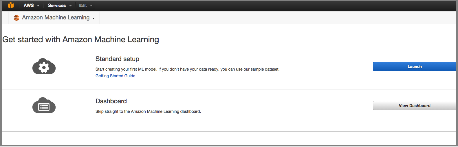
Starting Page: To start off, click on Dashboard from the Starting Page, and start creating your Data Source from your S3 bucket:

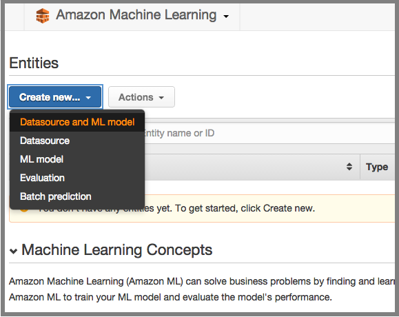
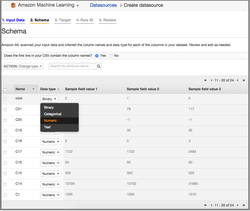
Data Source:

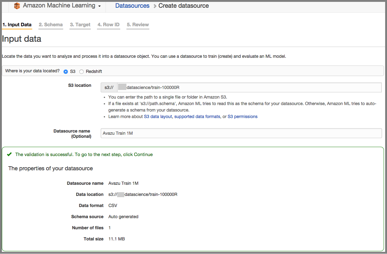
Load your training data from S3:

Note: Click should be changed into numeric since we expect the result to be probability. AML will then chose a Regression Model instead of Classification Model:

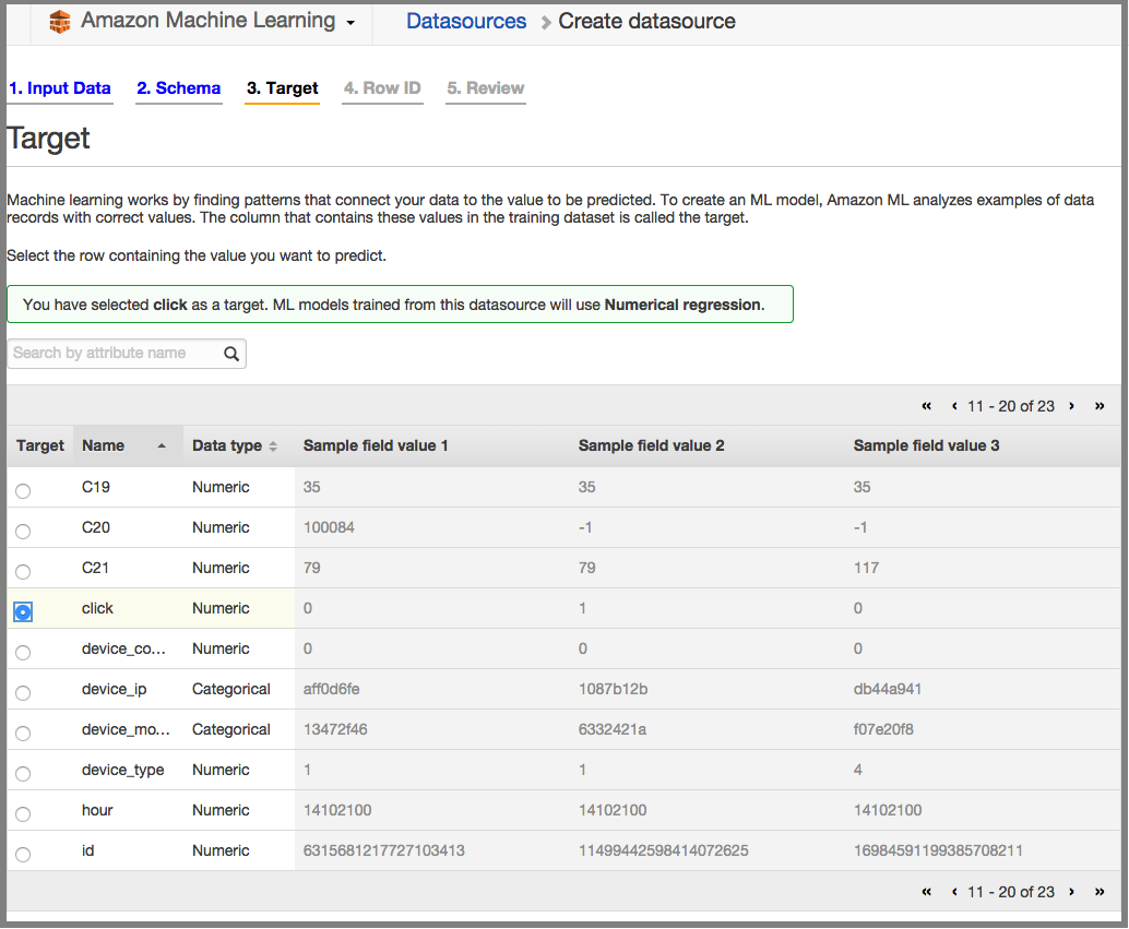
Chose Click as a target of the model:

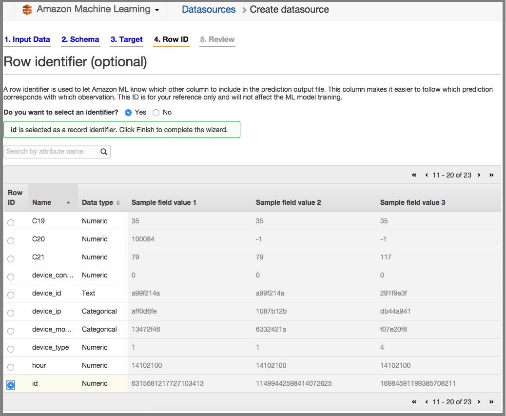
ID to be Row Identifier:

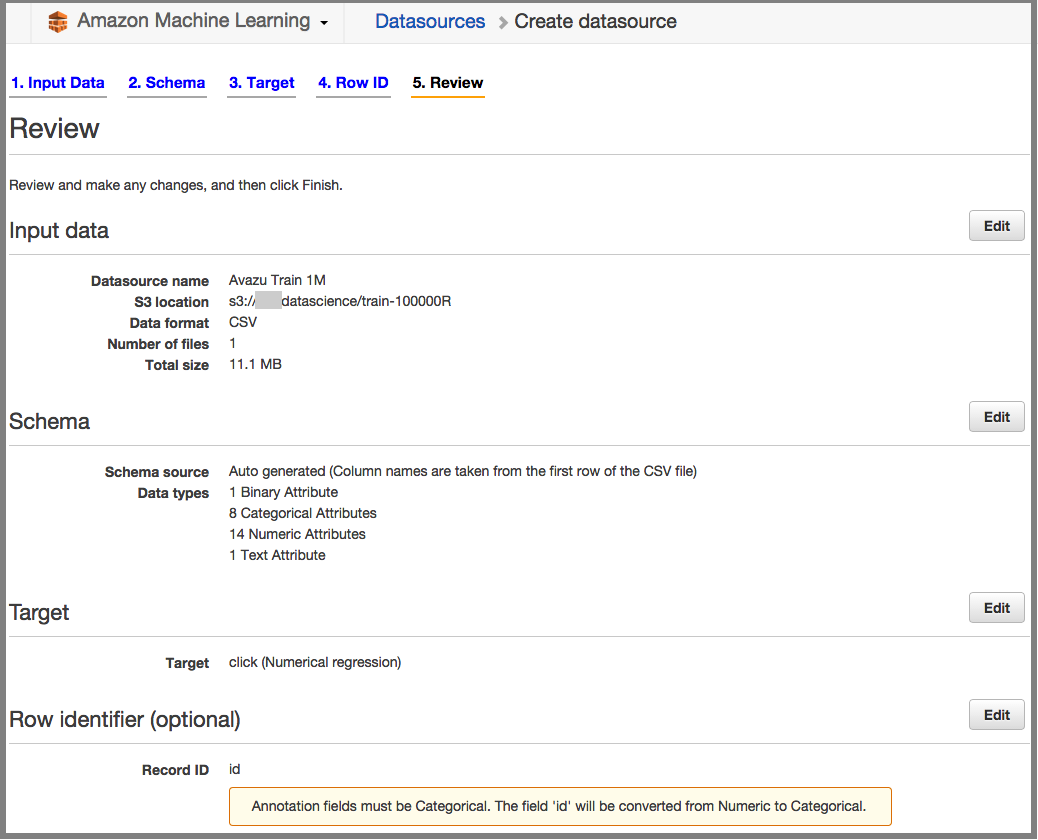
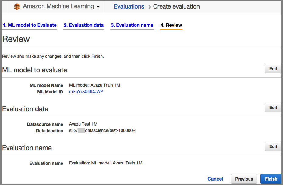
Review:

Data Model:

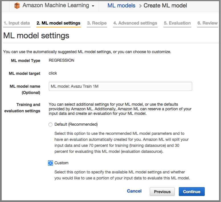
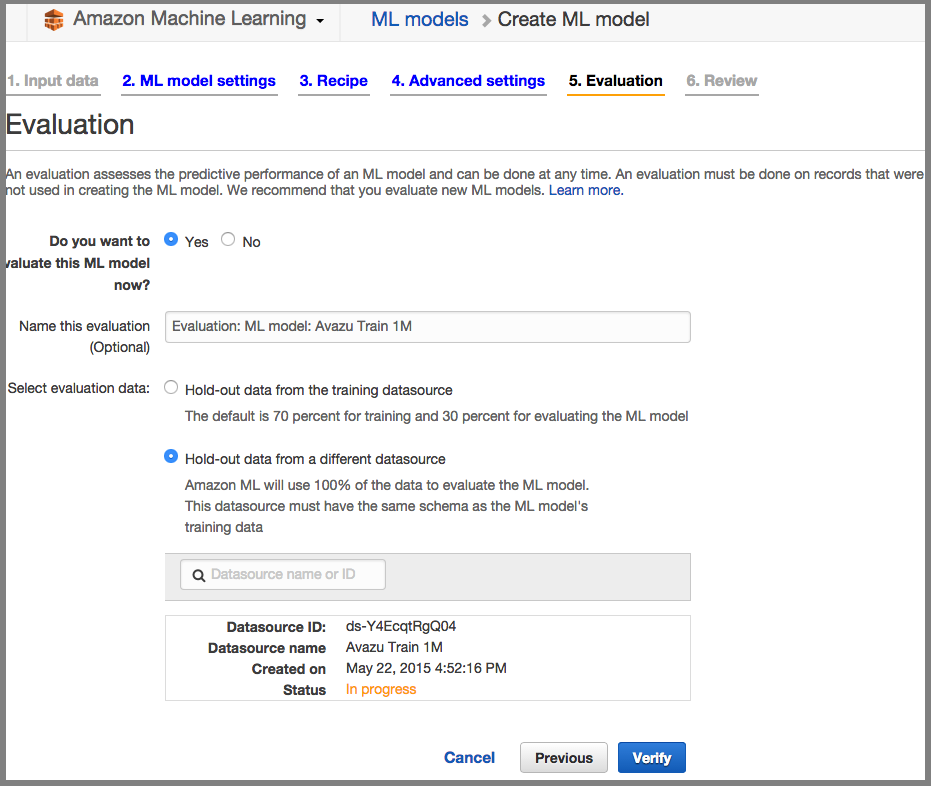
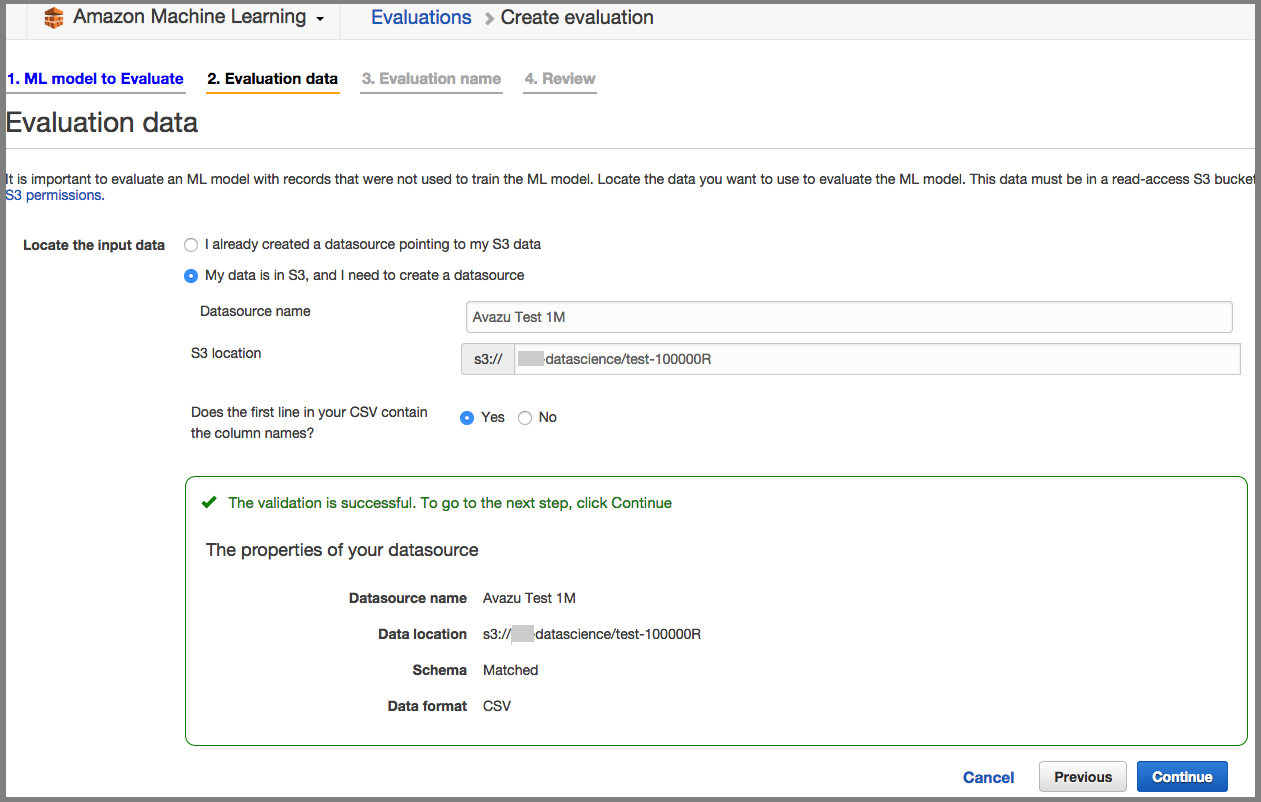
Chose “Hold-out data from a different datasource” since we already did it with test-100000R and train-100000R.

Review:

Evaluation:

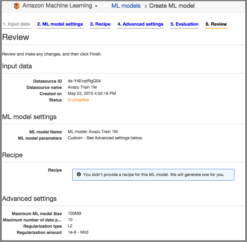
Review:

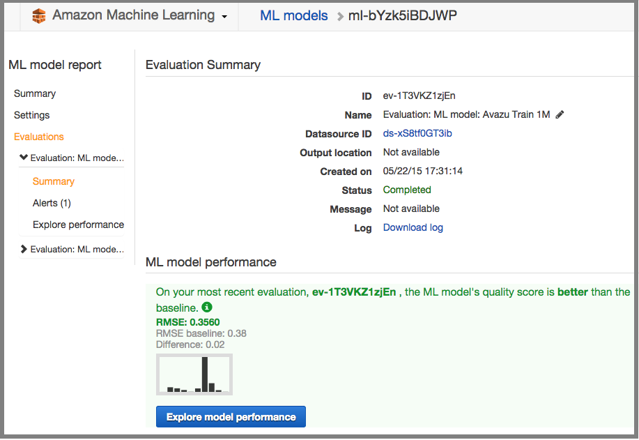
Summary:

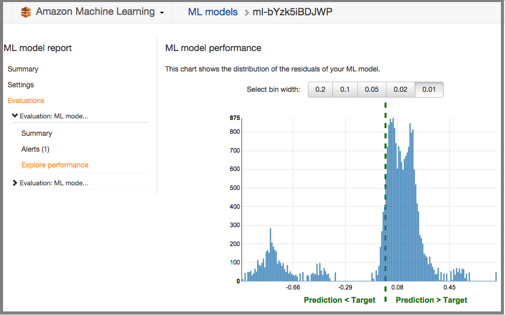
Overview - RMSE & Detailed Report.

Note: Amazon Machine Learning does not provide any other evaluation method for its regression model, apart from RMSE

Results, Pros and Cons

Results (The lower, the better)

Algorithm	Time Taken (s)	Log Loss	RMSE
Sklearn’s ExtraTreesClassifier	28.9	2.0065	0.4057
Sklearn’s RandomForestClassifier	57.6	0.7220	0.3802
Sklearn’s KNeighborsClassifier	2.4	0.4584	0.3780
Sklearn’s LDA	0.5	0.4372	0.3690
Sklearn’s GaussianNB	0.2	1.0092	0.4319
Sklearn’s DecisionTreeClassifier	3.8	7.3530	0.4729
Sklearn’s GradientBoostingClassifier	115.6	0.4168	0.3602
Sklearn’s SGDClassifier	0.8	0.4893	0.3921
AML’s Regression Model	600 (ish)	N/A	0.3560

Performance wise: Amazon’s Machine Learning (AML) clearly produced a better result than my best model, which scored better than half of the accepted submissions on Kaggle. AML is also extremely easy to use - it took me roughly 3 days to come up with a full implementation of my Scikit-Learn’s models, yet with AML, total time taken was less than 30 minutes.

Price wise: Creating a model cost almost nothing with AML (except for the time taken, which is quite long ~ 600 seconds, almost 6x comparing to Scikit-Learn’s slowest model!) However, keep in mind that it’s quite expensive to run your prediction, according to Amazon Machine Learning’s Pricing it cost $0.10 per 1000 batch predictions and $0.0001 per real-time prediction. This could end up to be quite expensive if you want to use AML for Kaggle competitions with a test set of 1 million entries ($100 for each submission!).

Practical wise: AML gives us a production-ready service, scalability and deployment should be easily done. This is, in my opinion, the best selling point of AML. In some cases, AML is not very flexibly configurable to your special or domain oriented business needs, but most of the case, I strongly think that it should give a very good baseline approach to solve busines’s data science problem effectively.